Policy Gradient Methods

Gradient Descent/Ascent is a great asset. If you have an approximation model consisting of some parameters $\theta$ and a cost function, $\mathcal{J}$ , then you can update the parameters $\theta$ with the gradient of $\mathcal{J}$ wrt to $\theta$ . In value approximation methods we try to approximate $V_\pi(s)$ or $Q_\pi(s,a)$ and we use a policy like $\epsilon$ -greedy for control. The problem with $\epsilon$ -greedy is that we have to choose a ‘max’ over all possible actions which is really time-consuming for enviroments with continous action space. Also, sometimes we need a stochastic policy like a Gaussian policy which would mostly choose actions around its mean but also ensures randomness in selection of an action. In such cases, its better to learn a policy for a particular environment that maximizes reward, and to do so we need gradients for our policy parameters. In this post we will look into different aspects of policy gradients and derive the necessary proofs.

Let’s choose a policy $\pi_\theta(s,a)$ with parameters $\theta$ . Gradients $\frac{\partial \mathcal{J}}{\partial \theta}$ depend on the choice of objective function. Formulating an objective function depends on the type of environment we are in. For an episodic environment:

$\begin{equation*} \mathcal{J}(\theta) = \mathbb{E}_{\pi_\theta} [V_{S_0}] \end{equation*}$

which basically translates to the expected reward from our starting state.

For continuous or a never ending environment we use a stationary distribution, $d_{\pi_\theta}(s)$ , which tells us distribution of states after the process has run for a sufficiently long time such that running the process anymore doesnt change the distribution. In such environments we look for averaging immediate rewards over the entire distribution states the we visit.

$\begin{equation*} \mathcal{J}(\theta) = \mathbb{E}_{\pi_\theta} [r] = \sum_{s \in \mathcal{S}} d_{\pi_\theta}(s) \sum_{a \in \mathcal{A}} \pi_\theta(a,s) r(s, a) \end{equation*}$

Let’s find policy gradients for both environments:

Episodic Environments:
Let’s say the probability of a trajectory $\tau$ as $\mathcal{P}(\tau \vert \theta)$ and the reward for the episode as $\mathcal{R}(\tau)$ . So put simply the total rewards here for an episode is the probability of the trajectory of the episode times the total end reward

$\begin{align*}\mathcal{J}(\theta) &= \mathcal{P}(\tau \vert \theta)\mathcal{R}(\tau) \\\nabla_\theta \mathcal{J}(\theta) &= \nabla_\theta \mathcal{P}(\tau \vert \theta)\mathcal{R}(\tau) \\&= \mathcal{P}(\tau \vert \theta) \nabla_\theta \ln \mathcal{P}(\tau \vert \theta) \mathcal{R}(\tau) && \end{align*}$

$\nabla_\theta \mathcal{P}(\tau \vert \theta)$ can be rewritten as $\mathcal{P}(\tau \vert \theta) \nabla_\theta \ln \mathcal{P}(\tau \vert \theta)$ since

(1) $\begin{equation*}\nabla_\theta \ln(x) = \frac{1}{x}\nabla_\theta(x) \end{equation*}$

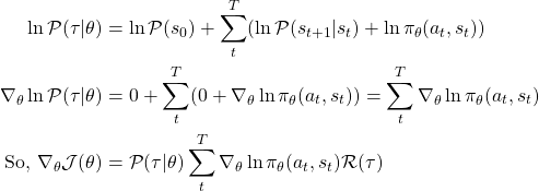
The probablility of a trajectory $\tau = (s_0,a_0,...s_{T+1})$ can be defined as:

$\begin{equation*} \mathcal{P}(\tau \vert \theta) = \mathcal{P}(s_0) \prod_{t}^{T} \mathcal{P}(s_{t+1} \vert s_t) \pi_\theta(a_t,s_t)\end{equation*}$

where $\mathcal{P}(s_0)$ is the probability of first state and $\mathcal{P}(s_{t+1} \vert s_t)$ is the probalility transition among states as governed by the environment. So,

$\begin{align*}\ln \mathcal{P}(\tau \vert \theta) &= \ln \mathcal{P}(s_0) + \sum_{t}^{T} (\ln \mathcal{P}(s_{t+1} \vert s_t) + \ln \pi_\theta(a_t,s_t)) \\\nabla_\theta \ln \mathcal{P}(\tau \vert \theta) &= 0 + \sum_{t}^{T} (0 + \nabla_\theta \ln \pi_\theta(a_t,s_t)) = \sum_{t}^{T} \nabla_\theta \ln \pi_\theta(a_t,s_t) \\\text{So, } \nabla_\theta \mathcal{J}(\theta) &= \mathcal{P}(\tau \vert \theta)\sum_{t}^{T}\nabla_\theta \ln \pi_\theta(a_t,s_t) \mathcal{R}(\tau)\end{align*}$

Now we formulated this loss for one episode. Lets say if we have D trajectories, then this turns into an expectation which we can estimate with sample mean.

(2) $\begin{align*}\nabla_\theta \mathcal{J}(\theta) &= \sum_{\tau}^{D}\mathcal{P}(\tau \vert \theta)\sum_{t}^{T}\nabla_\theta \ln \pi_\theta(a_t,s_t) \mathcal{R}(\tau) \nonumber \\&= \mathbb{E}_{\tau \sim \pi_\theta} [\sum_{t}^{T}\nabla_\theta \ln \pi_\theta(a_t,s_t) \mathcal{R}(\tau)] \\\end{align*}$

Continous Environments:
Using average reward per time step as our cost function,

$\begin{align*} \mathcal{J}(\theta) &= \sum_{s \in \mathcal{S}} d_{\pi_\theta}(s) \sum_{a \in \mathcal{A}} \pi_\theta(a,s) r(s, a)\end{align*}$

Finding gradients for continous environments is tricky. Changes in state distribution is a function of our policy as well as the environment. Since we dont know how environment works we dont know how our parameters $\theta$ affect $d_\pi(\theta)$ .

This is where policy gradient theorem comes in. Which says:

$\begin{equation*}\mathcal{J}(\theta) \propto \sum_{s \in \mathcal{S}} \mu(s) \sum_{a \in \mathcal{A}} \pi_\theta(a,s) q_\pi(s, a) \end{equation*}$

where, $\mu(s)$ is a distribution wherein $\mu(s) = \frac{\eta(s)}{\sum_s \eta(s)}$ ,which is a fraction of visits in that state divided by total visits in all states.
Also the proportionality constant is average length of episode in episodic environment and 1 in a continous environment.

$\begin{align*}\nabla_\theta \mathcal{J}(\theta) &= \sum_{s \in \mathcal{S}} \mu(s) \sum_{a \in \mathcal{A}} \nabla_\theta \pi_\theta(a,s) q_\pi(s, a) \\&= \sum_{s \in \mathcal{S}} \mu(s) \sum_{a \in \mathcal{A}} \pi_\theta(a,s) \nabla_\theta \ln \pi_\theta(a,s) q_\pi(s, a) && \text{Using (1)} \\&= \mathbb{E}_{\pi_\theta} [\nabla_\theta \ln \pi_\theta(a,s) q_\pi(s, a)] \end{align*}$

**Note**: The policy gradient theorem also works for episodic cases.

Compatible Function Approximation Theorem
If you notice the gradients have the term $q_\pi(s,a)$ and its true value is hard to come by so its easier to use a function approximator $q_w(s,a)$ to estimate it . But the question is wouldn’t it introduce bias is the estimation of gradients. As it turns out if you play cards right you can almost approximate the true gradients based on $q_\pi(s,a)$

So, the Compatible Function Approximation Theorem has these two conditions:
1) gradients of $q_w(s,a)$ = gradients of $\ln \pi_\theta(s,a)$

Mathematically,

(3) $\begin{equation*} \frac{\partial q_w(s,a)}{\partial w} = \frac{1}{\pi_\theta(s,a)}\frac{\partial \pi_\theta(s,a)}{\partial \theta} = \frac{\partial \ln \pi_\theta(s,a)}{\partial \theta}\end{equation*}$

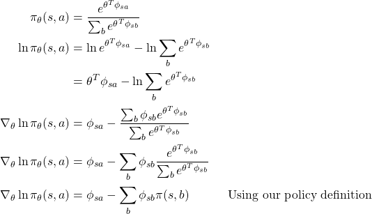
At first this condition seems bizzare like how can the gradients be same but it depends on the choice of the policy and the feature vectors used for value approximation. For example if you choose softmax policy after a linear transformation of feature vectors for discrete actions then the gradients of $\ln \pi_\theta(s,a)$ come out as:

$\begin{align*}\pi_\theta(s,a) &= \frac{e^{\theta^T \phi_{sa}}}{\sum_{b} e^{\theta^T \phi_{sb}}} \\\ln \pi_\theta(s,a) &= \ln e^{\theta^T \phi_{sa}} - \ln \sum_{b} e^{\theta^T \phi_{sb}} \\&= \theta^T \phi_{sa} - \ln \sum_{b} e^{\theta^T \phi_{sb}} \\\nabla_\theta \ln \pi_\theta(s,a) &= \phi_{sa} - \frac{\sum_{b} \phi_{sb} e^{\theta^T \phi_{sb}}}{\sum_{b} e^{\theta^T \phi_{sb}}} \\\nabla_\theta \ln \pi_\theta(s,a) &= \phi_{sa} - \sum_{b} \phi_{sb}\frac{ e^{\theta^T \phi_{sb}}}{\sum_{b} e^{\theta^T \phi_{sb}}} \\\nabla_\theta \ln \pi_\theta(s,a) &= \phi_{sa} - \sum_{b} \phi_{sb} \pi(s,b) &&\text{Using our policy definition} \end{align*}$

Now if choose our function approximator as:

$\begin{equation*} q_w(s,a) = w^T(\phi_{sa} - \sum_{b} \phi_{sb} \pi(s,b))\end{equation*}$

Then, $\partial_w q_w(s,a)$ = $\partial_\theta \ln \pi_\theta(s,a)$

2) We are minimizing least square error between true value functions and our function approximations.
We can get these true value function values using differnt policy evaluation methods. But lets see how this condition enables estimating true gradient values with function approximators that follow condition 1. Since we are minimizing the mesn squarred error in the estimation of all possible $q_\pi(s,a)$ values, so using a continous environment we get

$\begin{align*} \mathcal{U}_w &= \sum_{s \in \mathcal{S}} d_{\pi_\theta}(s) \sum_{a \in \mathcal{A}} \pi_\theta(a,s) (q_\pi(s,a) - q_w(s,a))^2 \\ \frac{\partial \mathcal{U}_w}{\partial w} &= 2 \sum_{s \in \mathcal{S}} d_{\pi_\theta}(s) \sum_{a \in \mathcal{A}} \pi_\theta(a,s) (q_\pi(s,a) - q_w(s,a))\frac{\partial q_w(s,a)}{\partial w} \\\end{align*}$

When this gradient reaches a local minimum then

$\begin{align*} 0 &= 2 \sum_{s \in \mathcal{S}} d_{\pi_\theta}(s) \sum_{a \in \mathcal{A}} \pi_\theta(a,s) (q_\pi(s,a) - q_w(s,a))\frac{\partial q_w(s,a)}{\partial w} \\0 &= \sum_{s \in \mathcal{S}} d_{\pi_\theta}(s) \sum_{a \in \mathcal{A}} \pi_\theta(a,s) (q_\pi(s,a) - q_w(s,a))\frac{\partial \ln \pi_\theta(s,a)}{\partial \theta} && \text{Using (3)} \\0 &= \sum_{s \in \mathcal{S}} d_{\pi_\theta}(s) \sum_{a \in \mathcal{A}} \pi_\theta(s,a) [\nabla_\theta \ln \pi_\theta(s,a) (q_\pi(s,a) - q_w(s,a)) ]\\0 &=\mathbb{E}_{\pi_\theta} [\nabla_\theta \ln \pi_\theta(s,a) (q_\pi(s,a) - q_w(s,a)) ] \\\mathbb{E}_{\pi_\theta} [\nabla_\theta \ln \pi_\theta(s,a) q_\pi(s,a)] &= \mathbb{E}_{\pi_\theta} [\nabla_\theta \ln \pi_\theta(s,a) q_w(s,a)]\end{align*}$

We can see now if both conditions are met then $q_w(s,a)$ gives a really good estimate of the true polciy gradients of $q_\pi(s,a)$ .

Advantage Function
Till now we talked about reducing bias when using function approximators but what about variance in our gradients. Lets say our environments have Reward or Qvalues of vary from 0 to 10000. This results a huge variance in gradients. A natural approach is to use concept called baselines. A baseline is a function that doesnt depend on the actions or in other words on our policy. A natural choice for baseline is $V_\pi(s)$ . Adding or substracting a baseline doesnt change the expectation of our gradients.

$\begin{align*} \mathbb{E}_{\pi_\theta} [\nabla_\theta \ln \pi_\theta(s,a) V_\pi(s)] &= \sum_{s \in \mathcal{S}} d_{\pi_\theta}(s) \sum_{a \in \mathcal{A}} \nabla_\theta \pi_\theta(a,s) V_\pi(s) \\&= \sum_{s \in \mathcal{S}} d_{\pi_\theta}(s)V_\pi(s) \sum_{a \in \mathcal{A}} \nabla_\theta \pi_\theta(a,s) \\&= \sum_{s \in \mathcal{S}} d_{\pi_\theta}(s)V_\pi(s) \nabla_\theta \sum_{a \in \mathcal{A}} \pi_\theta(a,s) \\&= 0\end{align*}$

So our advantage function looks like $A_\pi(s,a) = q_\pi(s,a) - V_\pi(s)$
In practise we estimate advantage function as $A(s,a) = q_w(s,a) - V_v(s)$ , using 2 seperate approximators and updating them using function approximation methods.

Related Posts

Leave a Comment Cancel Reply